Model Identification

This document is currently directly related to a project done in 2012 by Frane van Zyl, documented in the Model identification file.

System identification is the most expensive step in a model-based-control project.‭ ‬A study was therefore undertaken into model identification with the aim of understanding the fundamentals,‭ ‬and developing software tools that could be used to automate or ease the process.

Introduction

The process of system identification and the various model types were studied.‭ ‬A tool was written to perform the following steps present in any identification project:‭ (‬for all m-files see their headers for a description‭)

Experimental Design

A Psuedo Radom Binary Sequence was selected as the method to step the inputs in a multivariable fashion.‭ ‬Some more information on these and other steps are provided as‭ “‬PRBS and other step.pdf‭” ‬in the Reading Material folder on the CD of the project file.

The final matlab file is PRBS.m‭ (‬requires prbs.m‭)

Data Preparation

It is important that data be pre-filtered to remove outliers,‭ ‬trends and drift in the data.‭ ‬The function files written for this section is:

• Shift.m
• Normalise.m
• Expfilter.m
• Mavgfilter.m

More information is available from‭ ‬[‬http://upetd.up.ac.za/thesis/available/etd-07032009-170311/ Hernan Guidi,‭ ‬2008].‭

Estimation‭ (‬modelling phase‭)

Two choices need to be made:‭ ‬The type of model and the parameter estimation method.‭ ‬The ARX model and Laplace models were chosen,‭ ‬with the least squares regression as the‭ ‬estimation method.‭ ‬See Lyuben Chapter‭ ‬14‭ ‬for a good overview of some other techniques.‭

The basic idea behind ARX modelling is to write the ARX model:

$y(z) = \frac{B(z^{-1})}{A(z^{-1})} = \frac{\alpha_0 + \alpha_1 z^{-1} + \alpha_2 z^{-2} + \dots + a_m z^{-m}}{\beta_0 + \beta_1 z^{-1} + \beta_2 z^{-2} + \dots + \beta_m z^{-n}}$

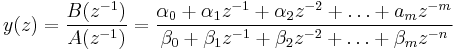
As a linear regression of the form Ax‭ = ‬b:

$y(t|\theta) = \phi^T\theta$

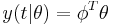
To solve for theta,‭ ‬we will need to find‭

$\theta = (\phi^T\phi)^{-1}\phi^T y$

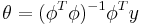
which involves the matrix inverse of‭ ‬$\phi$.‭ ‬That is if there exist an inverse and $\phi$ is not singular.‭ ‬It is far better therefore to use the pseudo-inverse‭ (‬see‭ ‬generalized-inverse‭) ‬or the left-inverse which is simply denoted by the operator,‭ \‬,‭ ‬in Matlab‭ (‬see‭ ‬left-inverse in Matlab‭)‬.‭ ‬Alternatively and reliably we can do a SVD,‭ ‬QR-decomposition,‭ ‬for a good overview of this see the following link:‭

http://classes.soe.ucsc.edu/cmps290c/Spring04/paps/lls.pdf

There are various texts on model identification using least squares and ARX modelling and the most informative was found as:

• Guidi,‭ ‬H.‭ (‬2008‭) “‬Open and Closed-loop Model Identification and Validation‭”‬,‭ ‬Masters Dissertation,‭ ‬Department of Chemical Engineering,‭ ‬University of Pretoria,‭ ‬Pretoria,‭ ‬South Africa.
• Morari,‭ ‬M.,‭ ‬Lee J.H.‭ & ‬Garcia E.,‭ ‬Model Predictive Control,‭ ‬March‭ ‬15,‭ ‬2002‭ [‬p1‭ ‬-‭ ‬101‭]‬.

The function files that perform the‭ ‬modelling and converstion to Laplace is given on the project CD as:

• ARX_MIMO_B.m
• ARXtoLaplace_MIMO.m
• validate_MIMO.m

Validation

Validation was chosen to be done by residual analysis‭ (‬plots and sum of the squares of the risiduals‭) ‬as well as predicted vs actual plots.

For the further reading on model validation,‭ ‬Hernan Guidi,‭ (‬2008‭) ‬gives a good overview,‭ ‬but there are also lots of general statistical material on the internet‭ ‬.‭)

The final functions written for model validation are provided on the project CD as:

• validate_SISO.m
• validate_MIMO.m

Simulation

A simulation is available from the Lab-Manual‭ (‬on the project CD‭) ‬that takes the student through the steps of model identification using a simulator.‭ ‬Matlab is required and the other software required for this can be downloaded free from:

• Prime5:‭ ‬http://www.randcontrols.co.za/downloads
• KEPserver:‭ ‬https://my.kepware.com/mykepware/‭ (‬register as a user first‭)